TABLE OF CONTENTS
・Euler method

Kaya
This time, let’s go over Euler’s method, a fundamental numerical integration technique for ordinary
differential equations.
Euler method
A differential equation in which the unknown function depends on only one variable is called an ordinary
differential equation (ODE).
Numerical integration of a differential equation refers not to solving it through indefinite
integrals, but rather to using appropriate approximation methods to obtain approximate solutions known as
numerical solutions.
Some differential equations cannot be solved in terms of indefinite integrals, or their solutions can only
be expressed using special functions.
In such cases, numerical integration becomes useful.

Nayumi
So the differential equations we’ve seen so far were just the basics…
Kaya
Yeah. There are all kinds of differential equations out there.

Nayumi
I see. So then, what kind of method is Euler’s method?
Kaya
Euler’s method is basically a reinterpretation of the definition of the derivative.
\[ \text{Euler method}\]
The Euler method is one of the numerical integration methods for ordinary differential
equations.
For an unknown function \( y = f(x) \), suppose that its derivative function \( y' = f'(x) \) is known.
Assuming \( n \) is a natural number, \( h \) is the step size, and the initial value is \( \left(
x_0,y_0 \right) \), the numerical solution \( \left( x_n,y_n \right) \) is obtained as follows.
\[ \begin{align}
x_n &= x_{n-1} + h \\\\
y_n &= y_{n-1} + hf'(x_{n-1})
\end{align}\]
Nayumi
Where exactly is the derivative in this?
Kaya
If you rewrite \( y_n \) a little, you’ll see.
\[ \begin{align}
y_n &= y_{n-1} + hf'(x_{n-1}) \\\\
y_n - y_{n-1} &= hf'(x_{n-1}) \\\\
\frac{y_n - y_{n-1}}{h} &= f'(x_{n-1}) \\\\
f'(x_{n-1}) &= \frac{y_n - y_{n-1}}{h}
\end{align}\]
Kaya
Let’s line this up with the definition of the derivative at \( x_{n-1} \).
Euler method
\[ f'(x_{n-1}) = \frac{y_n - y_{n-1}}{h} \]
The derivative at \( x_{n-1} \)
\[ \begin{align}
f'(x_{n-1}) &= \lim_{h \to 0} \frac{f(x_{n-1}+h) - f(x_{n-1})}{h} \\\\
&= \lim_{h \to 0} \frac{f(x_{n}) - f(x_{n-1})}{h}
\end{align} \]
If we regard \( y_n = f(x_n) \), Euler’s method and the definition of the derivative at \( x_{n-1} \) are
essentially the same, except for the presence or absence of the limit notation.
Euler’s method deliberately treats \( h \) not as the limit \( h \to 0 \) in the definition of the
derivative, but as a finite step size, which makes it possible to compute the value of \( y_n \) from the
initial value.
Nayumi
What does it actually look like when you try it out?
Kaya
Good question. Let’s look at an example using Euler’s method on \( y = \frac{1}{4} x^2 \). Starting from
\( \left( x_0,y_0 \right) = (0,0) \), and for clarity, we’ll use a relatively large step size of \( h =
\frac{1}{2} \).
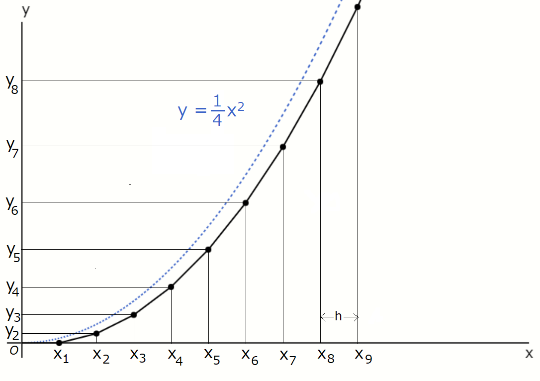
The black line represents the numerical solution obtained with Euler’s method, while the blue dashed line
shows the true solution \( y = \frac{1}{4} x^2 \).
What Euler’s method actually computes are the black dots; the black line connecting them is just drawn for
clarity, so keep that in mind.
Nayumi
In this example, the Euler method results are a bit off from the exact values, but if we use a smaller
step size, we can get a more accurate result, right?
Kaya
Exactly. If we take the step size as \( h = \frac{1}{10} \), it looks like this.
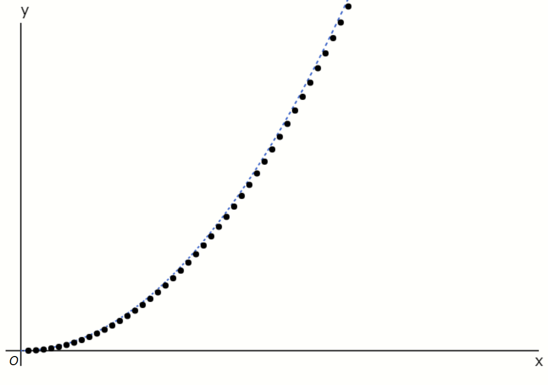
The error between the numerical solution \( y_n \) obtained by Euler’s method and the exact value is known
to be roughly proportional to the step size \( h \).
However, making the step size smaller increases the number of calculations, and when computing on a
computer, rounding errors (round-off errors) also become more significant. So, smaller is not always
better.
From the perspective of keeping computation time short, using an excessively small step size that
drastically increases the number of calculations is also undesirable. Therefore, it is important to choose
an appropriate step size.
Nayumi
Actually performing the calculations is pretty tricky, isn’t it?

Kaya
Yeah. There are many small points to watch out for, but numerical integration is still an effective way
to investigate solutions of differential equations. In the future, you’ll likely use numerical
integration in numerical experiments to find solutions, so get used to it.
Nayumi
Got it.
Finally, Leonhard Euler, who devised Euler’s method, was an 18th-century mathematician born in Switzerland.
He laid the foundations for many areas of mathematics and physics, and numerous theorems and equations bear
his name—Euler’s method is just one of them.

Leonhard Euler(1707-1783)
References:
[1] Euler method, https://en.wikipedia.org/wiki/Euler_method, August
14, 2023
[2] オイラー法の誤差について, https://hinabit.hatenablog.com/entry/2015/02/13/015201,
August 14, 2023
[3] Stanley J. Farlow, Partial Differential Equations for Scientists and Engineers, Dover Publications,
September 1, 1993
[4] Wikipedia Leonhard Euler, https://en.wikipedia.org/wiki/Leonhard_Euler,
August 22, 2025
Previous
Ep. 8
Indefinite integral
Next
Ep. 10
Increase/Decrease and extrema