Ep. 2  Function of one variable

Mathematics articles that help in reading this article
・Numerical Computation：Ep. 1

　A relationship \( f \) in which the value of variable \( y \) is uniquely determined by the value of a single variable \( x \) is called a function of one variable, and it is expressed as \( y = f(x) \). In this context, \( x \) is called the independent variable, and \( y \) is called the dependent variable. The range of values that \( x \) can take is called the domain, and the range of values that \( y \) can take is called the image. Unless otherwise specified, the domain is often assumed to be all real numbers.

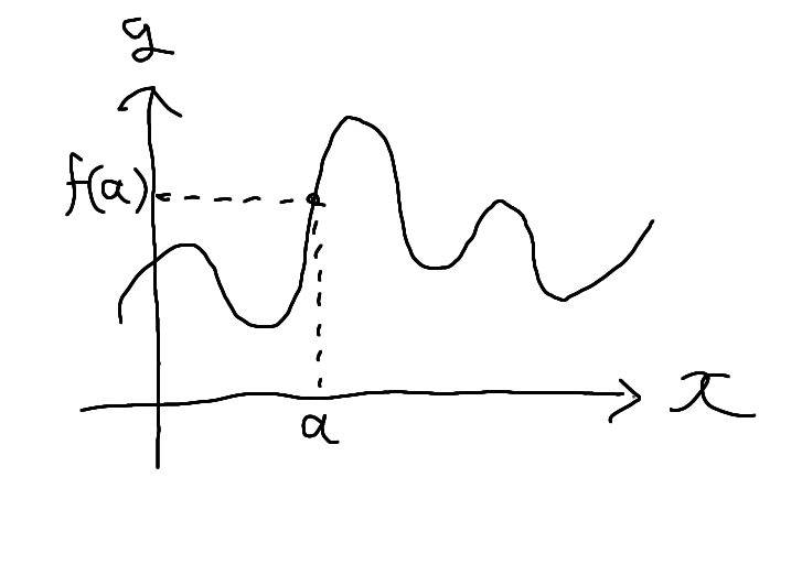
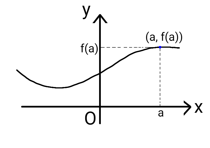
　For the function \( y = f(x) \), the set of all points \( (x, y) \) that satisfy this relationship is called the graph of the function \( y = f(x) \). When illustrated, the graph appears as shown below, where the value \( a \) on the \( x \)-axis corresponds to the value \( f(a) \) on the \( y \)-axis. The symbol \( O \) written at the intersection of the \( x \)-axis and the \( y \)-axis represents the origin, which corresponds to the point \( (x, y) = (0, 0) \).

　The phrase “as \( x \) approaches \( a \) without actually reaching \( a \)” in the definition of a limit cleverly avoids the subtle issues related to zero.

　For example, let's consider the process of finding instantaneous speed. We obtain the instantaneous speed by making the time interval \( \Delta t \) for average speed infinitely small. But what happens if we set this time interval \( \Delta t = 0 \)? If the time interval is \( 0 \), it means no time has passed, so the change should be stopped. In this case, the instantaneous speed would be \( 0 \). However, with this reasoning, since no time is passing at any moment, the instantaneous speed would always be \( 0 \), and no change would occur.

　This idea is a generalization of the paradox "The arrow in flight does not move," which is attributed to the ancient Greek philosopher Zeno. Zeno argued that at every instant of the flying arrow, if you isolate that moment, the arrow is stationary, and thus, he claimed that the flying arrow is always at rest. It is a bit of a sophistry, but when we start considering the time interval \( \Delta t = 0 \), we inevitably face such paradoxical reasoning. To avoid confronting this problem, the definition of a limit, as we saw earlier, is used.

　The key point of the definition of the limit is that the expression "approaching \( a \)" focuses not on how close you get to a certain number, but on the process of getting closer and closer to that number.

　In most numerical experiments, the functions we deal with are continuous over all real numbers, so we usually don’t need to worry much about the continuity of the function. However, the continuity of functions is an important concept to remember, as it plays a key role in the proofs of various theorems that will appear later.
　To give an example of a function that is not continuous, there is the floor function.

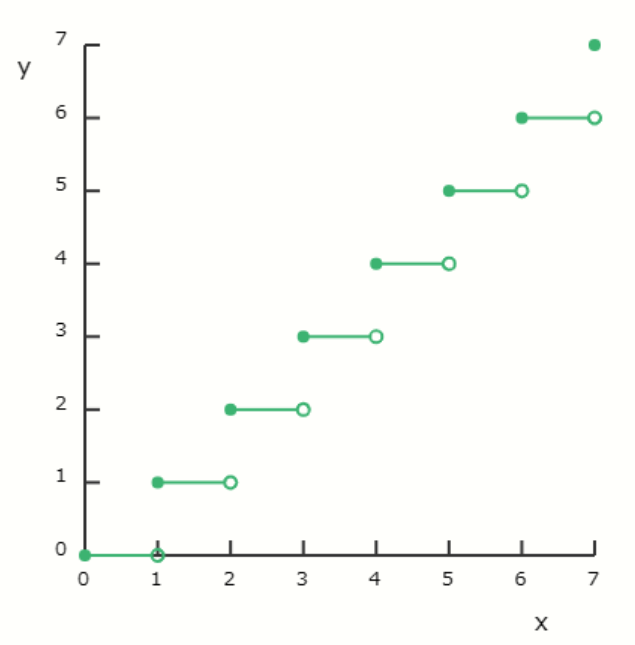
　The graph of the floor function is discontinuous at \( x = n \) (where \( n \) is an integer). The gaps on the right side occur because the floor function "cuts off" the decimal part.
　If \( x \) is slightly greater than an integer, the floor function gives the value of that integer. However, if \( x \) is slightly smaller than an integer, the floor function gives the integer just below it. To visualize it, think of the floor function as the floor of a building at the height of an integer, where the objects inside the building are classified according to the floor they are directly beneath.

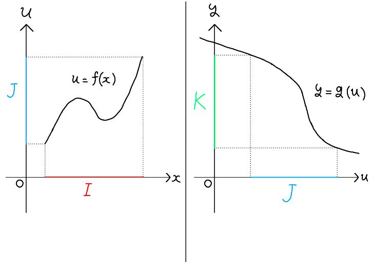
　If there are two functions \( u = f(x) \) and \( y = g(u) \), and the image of \( u = f(x) \) is included in the domain of \( y = g(u) \), then the function \( y = g(f(x)) \) can be defined, which is called the composite function of \( f \) and \( g \).
　The domain of the composite function \( y = g(f(x)) \) is the same as the domain of \( u = f(x) \) (denoted \( I \) in the figure). Its range is equal to the range of \( y = g(u) \) when the domain of \( g \) is taken to be the range of \( u = f(x) \) (denoted \( J \) in the figure). The resulting range is denoted \( K \).

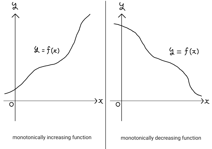
　For a function \( y = f(x) \), if \( f(a) \leq f(b) \) holds for all \( a \leq b \) in its domain, we say that \( f(x) \) is a monotonically increasing function. Conversely, if \( f(a) \geq f(b) \) holds for all \( a \leq b \) in its domain, we say that \( f(x) \) is a monotonically decreasing function.

　Let \( y = f(x) \) be a continuous and monotonic (increasing or decreasing) function on its domain. In this case, the function that assigns \( x \) to each \( y \) is called the inverse function of \( y = f(x) \), and is denoted by \( x = f^{-1}(y) \). Alternatively, by interchanging \( x \) and \( y \), it can be written as \( y = f^{-1}(x) \).
　The graph of \( y = f(x) \) becomes the graph of \( x = f^{-1}(y) \) when reflected across the line \( y = x \).

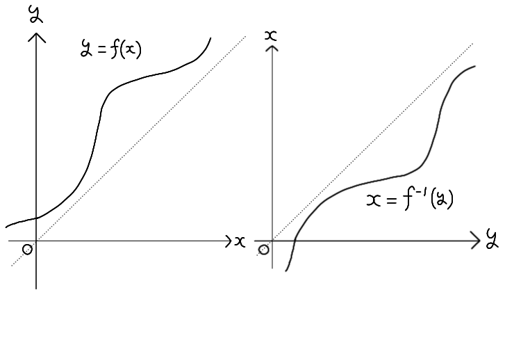
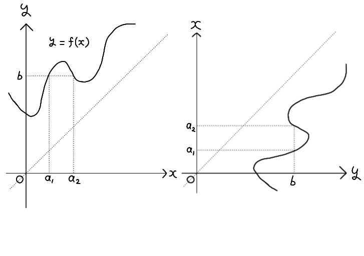
　Also note that if \( y = f(x) \) is not monotonic (increasing or decreasing) on its domain, then for some values of \( y \), the corresponding value of \( x \) is not uniquely determined, and therefore an inverse function cannot be defined.

References:

[1] Wikipedia Zeno's paradoxes, https://en.wikipedia.org/wiki/Zeno%27s_paradoxes、July
15, 2023
[2] 森毅, 位相のこころ, 筑摩書房, January 10, 2006
[3] 石村園子, やさしく学べる微分積分, 共立出版, December 25, 1999
[4] 難波 誠, 数学シリーズ 微分積分学, 裳華房, January 20, 2009
Previous
Ep. 1
Numbers
Next
Ep. 3
Straight line and
conic section