TABLE OF CONTENTS
・Exponent
・Exponential function
・Logarithm
・Logarithmic function
Kaya
This time, let's go over exponential and logarithmic functions.
Exponent
\[ \text{Power}\]
An expression formed by multiplying the same variable, constant, or number repeatedly is called a
power.
The number of multiplications is written as a superscript to the right of the base.
For example:
\[ a \times a \times a = a^3\]
The variable, constant, or number being multiplied is called the base, and the number of times it
is multiplied is called the exponent.
The process of applying a power to a base, resulting in repeated multiplication of the base, is called
exponentiation.
Nayumi
Oh, so it makes things easier when you're multiplying the same number over and over.
Kaya
Yeah. It's especially useful when dealing with large numbers. The next part gives a more precise
definition of powers of positive real numbers.
\[ \text{Powers of positive real numbers}\]
When \( a \) is a positive real number, \( n \) is a natural number, and \( m \) is an integer, the
powers of \( a \) are defined as follows:
[1] \( a^0 = 1 \)
[2] \( a^n \) is equal to multiplying \( a \) by itself \( n \) times.
[3] \( a^{-n} \) is equal to multiplying \( \frac{1}{a} \) by itself \( n \) times.
[4] \( a^{\frac{m}{n}} \) is the \( n \)th root of \( a^m \), i.e., the number that, when multiplied by itself \( n \) times, gives \( a^m \). This is expressed as: \[ a^{\frac{m}{n}} = \sqrt[n]{a^m}\] Particularly, when \( n = 2 \), it may be simplified to: \[ a^{\frac{m}{2}} = \sqrt{a^m}\] [5] When \( p \) is an irrational number and \( \{ p_l \} \) is a sequence of rational numbers with: \[ \lim _{l \to \infty} p_l = p\] then the power of \( a \) raised to the irrational exponent \( p \) is defined as: \[ a^p = \lim _{l \to \infty} a^{p_l}\]
The meaning of definition [1] above becomes clear when we consider the following limit.
\[ \lim _{n \to \infty} a^{\frac{1}{n}} \ \ (a \gt 0) \]
The symbol \( \infty \) represents infinity.
\[ \lim_{n \to \infty}\]
means that \( n \) is becoming infinitely large.
According to [4], \( a^{\frac{1}{n}} \) represents the \( n \)th root of \( a \)—that is, the number which,
when multiplied by itself \( n \) times, equals \( a \).
As \( n \) increases, \( a^{\frac{1}{n}} \) approaches 1. In other words, the following equation holds:
\[ \lim _{n \to \infty} a^{\frac{1}{n}} = 1 \ \ (a \gt 0) \]
And since \( n \to \infty \) implies that \( \frac{1}{n} \to 0 \), this limit can also be written as
follows, and it means the same thing.
\[ \lim _{n \to 0} a^{n} = 1 \ \ (a \gt 0) \]
From the fact that this limit holds, the definition in [1] is adopted for powers of positive real numbers.
Nayumi
I see now what 0 raised to a power means.
Kaya
The remaining part is [5].
[5] defines exponentiation when the exponent is an irrational number.
[4] only allows us to define exponentiation when the exponent is a rational number—that is, when it can be
expressed as a fraction with integer numerator and denominator—so [5] is necessary.
In [5], the term sequence appears. As the word suggests, this refers to a list of numbers arranged in a sequence. Each number in the list is called a term. A sequence is typically written as: \[ a_1,\ a_2,\ a_3,\ \ldots,\ a_n,\ \ldots\] In this case, \( a_1 \) is called the first term. A sequence can also be written as \( \{ a_n \} \).
Like functions, sequences are often analyzed using limits, which are defined as follows.
\[ \text{Limit of a sequence}\]
For a sequence \( \{ a_n \} \), if for any arbitrarily small positive number \( \epsilon \), there
exists a number \( M \) such that for all terms beyond the \( M \)th term, the absolute
difference between \( a_n \) and \( a \) is smaller than \( \epsilon \), then the sequence \( \{ a_n \}
\) is said to converge, and its limit is \( a \). This is expressed as:
\[ \lim _{n \to \infty} a_n = a \]
\( \epsilon \) is read as "epsilon."
The absolute value, put simply, is a number with its minus sign removed.
More formally, it is defined as follows:
\[ \text{Absolute value}\]
The absolute value of the real number \( a \) is equal to \( a \) if \( a \) is greater than or
equal to 0, and equal to \( -a \) if \( a \) is less than 0.
The absolute value of \( a \) is denoted by \( |a| \) .
To deepen our understanding of the convergence of sequences, let's consider the following specific example.
\[ 1, \frac{1}{10} , \frac{1}{100} , \frac{1}{1000}, \ldots \]
The limit of this sequence is \( 0 \).
For example, if we take \( \epsilon = \frac{2}{10} \), then the value of \( M \) in the definition becomes
1.
Similarly, if \( \epsilon = \frac{2}{100} \), then \( M \) becomes 2.
The key point is that no matter how small \( \epsilon \) gets, we can always choose a corresponding \( M \).
Nayumi
So [5] is basically saying: let's express an exponent that's an irrational number as the limit of a
sequence of rational numbers.
But is it really that easy to construct a sequence of rational numbers that converges to some arbitrary
irrational number \( p \) we've chosen?
Kaya
It might not be easy, but it can be done.
There are various ways to construct sequences of rational numbers that converge to an irrational number.
For example, using the bisection method, we can in principle compute any value of the form \(
\sqrt[\frac{m}{n}]{a} \), where \( a \) is a positive rational number, \( n \) is a natural number, and \( m
\) is an integer.
The sequence of rational numbers generated in the process of this calculation will converge to the
irrational number being approximated by the bisection method.
Pi \( (\pi) \) is also an irrational number, but there are many known sequences of rational numbers that
converge to \( \pi \).
So, there's no need to worry about whether a rational sequence converging to a given irrational number
exists—it always does.
Nayumi
So there's nothing to worry about, then.
Kaya
Exactly. Now that we've defined exponentiation, let's move on to explaining the laws of exponents.
\[ \text{Laws of exponents}\]
In calculations involving exponents, the following laws of exponents hold true for positive real
numbers \( a \) and \( b \), and real numbers \( p \) and \( q \):
\[ \begin{align}
&[1]\ a^p a^q = a^{p+q} \\
&[2]\ \left( a^p \right) ^q = a^{pq} \\
&[3]\ (ab)^p = a^p b^p \\
&[4]\ \frac{a^p}{a^q} = a^{p-q} \\
&[5]\ \left( \frac{1}{a^p} \right) ^q = \frac{1}{a^{pq}} \\
&[6]\ \left( \frac{a}{b} \right) ^p = \frac{a^p}{b^p}
\end{align} \]
Since proving the laws of exponents for real numbers \( p \) and \( q \) is a bit more difficult, we will
prove them here only for the case where \( p \) and \( q \) are rational numbers.
\[ \text{Proof of the law of exponents [1]}\]
Let \( l \) and \( n \) be natural numbers, and let \( k \) and \( m \) be integers.
\[ \begin{align}
a^{\frac{m}{n}} a^{\frac{k}{l}} &= \sqrt[n]{a^m} \sqrt[l]{a^k} \\\\
&= \sqrt[ln]{a^{lm}} \ \sqrt[ln]{a^{kn}} \\\\
&= \sqrt[ln]{a^{lm} a^{kn}} \\\\
&= \sqrt[ln]{a^{lm+kn}} \\\\
&= a^{\frac{lm+kn}{ln}} \\\\
&= a^{\frac{m}{n} + \frac{k}{l}}
\end{align} \]
\[ \text{Proof of the law of exponents [2]}\]
Let \( l \) and \( n \) be natural numbers, and let \( k \) and \( m \) be integers.
\[ \begin{align}
\left( a^{\frac{m}{n}} \right) ^{\frac{k}{l}} &= \sqrt[l]{\left( a^{\frac{m}{n}} \right) ^k} \\\\
&= \sqrt[l]{a^{\frac{km}{n}}} \\\\
&= a^{\frac{km}{ln}}
\end{align} \]
\[ \text{Proof of the law of exponents [3]}\]
Let \( n \) be natural numbers, and let \( m \) be integers.
\[ \begin{align}
\left( ab \right) ^{\frac{m}{n}} &= \sqrt[n]{\left( ab \right) ^m} \\\\
&= \sqrt[n]{a^m b^m} \\\\
&= \sqrt[n]{a^m}\ \sqrt[n]{b^m} \\\\
&= a^{\frac{m}{n}}\ b^{\frac{m}{n}}
\end{align} \]
\[ \text{Proof of the law of exponents [4]}\]
Let \( l \) and \( n \) be natural numbers, and let \( k \) and \( m \) be integers.
\[ \begin{align}
\frac{a^{\frac{m}{n}}}{a^{\frac{k}{l}}} &= \frac{\sqrt[n]{a^m}}{\sqrt[l]{a^k}} \\\\
&= \frac{\sqrt[ln]{a^{lm}}}{\sqrt[ln]{a^{kn}}} \\\\
&= \sqrt[ln]{\frac{a^{lm}}{a^{kn}}} \\\\
&= \sqrt[ln]{a^{lm-kn}} \\\\
&= a^{\frac{lm-kn}{ln}} \\\\
&= a^{\frac{m}{n}-\frac{k}{l}} \\\\
\end{align} \]
\[ \text{Proof of the law of exponents [5]}\]
Let \( l \) and \( n \) be natural numbers, and let \( k \) and \( m \) be integers.
\[ \begin{align}
\left( \frac{1}{a^{\frac{m}{n}}} \right) ^{\frac{k}{l}} &= \left( a^{-\frac{m}{n}} \right)
^{\frac{k}{l}} \\\\
&= \left( a^{-\frac{km}{ln}} \right) \\\\
&= \frac{1}{a^{\frac{km}{ln}}}
\end{align} \]
\[ \text{Proof of the law of exponents [6]}\]
Let \( n \) be natural numbers, and let \( m \) be integers.
\[ \begin{align}
\left( \frac{a}{b} \right) ^{\frac{m}{n}} &= \sqrt[n]{\left( \frac{a}{b} \right) ^{m}} \\\\
&= \sqrt[n]{a ^{m}} \ \sqrt[n]{\left( \frac{1}{b} \right) ^{m}} \\\\
&= a^{\frac{m}{n}} \times \left( \frac{1}{b} \right) ^{\frac{m}{n}} \\\\
&= \frac{a^{\frac{m}{n}}}{b ^{\frac{m}{n}}}
\end{align} \]
Nayumi
That was pretty long.
Kaya
Good work. Let's wrap up exponents here and move on to exponential functions.
Exponential function
Nayumi
Is an exponential function just a function with an exponent?
Kaya
That's right. An exponential function is defined as follows.
\[ \text{Exponential function}\]
Suppose that \( a \) is a positive real number.
The function \[ y = a^x \] is called an exponential function with base \( a \).
Nayumi
Hmm, what does the graph of this function look like?
Kaya
Good question. Let's try plotting the graph using two examples: \( a = 2 \) and \( a = \frac{1}{2} \).
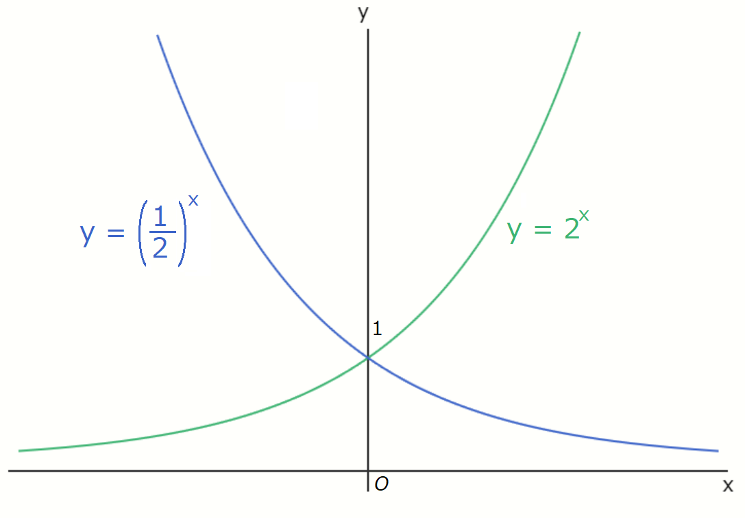
Here, we used \( y = 2^x \) and \( y = \left( \frac{1}{2} \right)^x \) as examples, but in general, the
graphs of \( y = a^x \) and \( y = \left( \frac{1}{a} \right)^x \) are symmetric with respect to the \( y
\)-axis.
Also, both graphs pass through the point \( (0, 1) \), which is because any positive real number raised to
the power of 0 equals 1.
Furthermore, regardless of the value of the base, the range of an exponential function is the set of all
positive real numbers, so its graph always lies above the \( x \)-axis.
Kaya
To wrap up our discussion on exponential functions, let's define the number \( e \), known as Euler's
number.
\[ \text{Euler's number}\]
The exponential function whose tangent slope (derivative) at \( x = 0 \) is \( 1 \) is expressed
as
\[ y = e^x \]
where \( e \) is called the Euler's number or Napier's constant.
The following limit formulas hold for \( e \): \[ \lim _{x \to 0} \frac{e^x - 1}{x} = 1 \] \[ \lim _{x \to 0} \left( 1+x \right) ^{\frac{1}{x}} = e \]
The following limit formulas hold for \( e \): \[ \lim _{x \to 0} \frac{e^x - 1}{x} = 1 \] \[ \lim _{x \to 0} \left( 1+x \right) ^{\frac{1}{x}} = e \]
Euler's number, denoted \( e \), is an irrational number approximately equal to \( 2.71828\ldots \).
A tangent line, in simple terms, is a straight line that just barely touches a curve.
More precisely, it is a line that shares exactly one point with the curve and has the same slope as the
curve at that point.
Kaya
Alright, that wraps up exponential functions—now let's move on to logarithms.
Logarithm
Nayumi
Logarithm?
Kaya
You can think of a logarithm as the reverse operation of exponentiation.
\[ \text{Logarithm}\]
The logarithm of \( b \) with base \( a \) is the exponent \( n \) that satisfies \( a^n = b \),
expressed as:
\[
\log _{a} b = n
\]
Here, \( b \) is called the antilogarithm (or argument). The base \( a \) must be a
positive real number other than 1, and \( b \) must be a positive real number.
The logarithm with base 10 is called the common logarithm, while the logarithm with base \( e =
2.71828 \dots \) is called the natural logarithm. The common logarithm is often denoted as \(
\log b \), and the natural logarithm as \( \ln b \).
The base of a logarithm is required to be a positive real number not equal to 1, since 1 raised to any
power always equals 1, which would make the logarithm undefined or meaningless in most contexts.
Kaya
There are several rules for calculating with logarithms.
\[ \text{Logarithmic laws}\]
For \( a > 0 \), \( a \neq 1 \), \( p > 0 \), \( q > 0 \), and any real number \( r \), the following
logarithmic laws hold:
\[
\begin{align}
&[1]\ \log _{a} (pq) = \log _{a} p + \log _{a} q \\
&[2]\ \log _{a} \frac{1}{q} = - \log _{a} q \\
&[3]\ \log _{a} \frac{p}{q} = \log _{a} p - \log _{a} q \\
&[4]\ \log _{a} q^r = r \log _{a} q \\
\end{align}
\]
All logarithmic laws can be derived from the laws of exponents.
Here, we will assume that the laws of exponents hold for real exponents and use that assumption to prove the
logarithmic laws.
\[ \text{Proof of logarithmic law [1]}\]
By the definition of logarithms,
\[ a^{\log _a p} = p\]
\[ a^{\log _a q} = q\]
Therefore,
\[ pq = a^{\log _a p} \times a^{\log _a q} = a^{\log _a p + \log _a q}\]
On the other hand, by the definition of logarithms,
\[ a^{\log _a pq} = pq \]
So we have:
\[ a^{\log _a pq} = a^{\log _a p + \log _a q}\]
Taking the logarithm with base \( a \) of both sides, we get:
\[ \log _a pq = \log _a p + \log _a q\]
\( \log_a p \) is the number that answers the question, "To what power must \( a \) be raised to get \( p
\)?"
Therefore, \( a^{\log_a p} \), which brings that number as the exponent of \( a \), naturally equals \( p
\).
By finding \( pq \) in two different ways and equating the results, we have derived the first logarithmic
law.
Nayumi
"We used the method of finding the same thing in two different ways and equating them to derive the
formula, just like with the sum formula for trigonometric functions.
Kaya
That's right. Now, let's move on to [2].
\[ \text{Proof of logarithmic law [2]}\]
By the definition of logarithms,
\[ a^{\log _a q} = q\]
Therefore,
\[ a^{-\log _a q} = \frac{1}{q}\]
On the other hand, by the definition of logarithms,
\[ a^{\log _a \frac{1}{q}} = \frac{1}{q} \]
So we have:
\[ a^{\log _a \frac{1}{q}} = a^{-\log _a q}\]
Taking the logarithm with base \( a \) of both sides, we get:
\[ \log _a \frac{1}{q} = -\log _a q\]
Nayumi
Hmm, in the second line, you used a negative exponent.
Kaya
That's right. After that, the method is the same as [1]. Now, let's move on to the proof of [3].
\[ \text{Proof of logarithmic law [3]}\]
By the definition of logarithms,
\[ a^{\log _a p} = p\]
From logarithmic law [2],
\[ a^{\log _a \frac{1}{q}} = a^{-\log _a q} = \frac{1}{q}\]
Therefore,
\[ \frac{p}{q} = a^{\log _a p} \times a^{-\log _a q} = a^{\log _a p - \log _a q} \]
On the other hand, by the definition of logarithms,
\[ a^{\log _a \frac{p}{q}} = \frac{p}{q} \]
So we have:
\[ a^{\log _a \frac{p}{q}} = a^{\log _a p - \log _a q} \]
Taking the logarithm with base \( a \) of both sides, we get:
\[ \log _a \frac{p}{q} = \log _a p - \log _a q\]
Nayumi
It's very similar to the proof of [1].
Kaya
That's right. Finally, let's prove logarithmic law [4].
\[ \text{Proof of logarithmic law [4]}\]
By the definition of logarithms,
\[ a^{\log _a q} = q\]
Therefore,
\[ q^r = \left( a^{\log _a q} \right)^r = a^{r \log _a q}\]
On the other hand, by the definition of logarithms,
\[ a^{\log _a q^r} = q^r \]
So we have:
\[ a^{\log _a q^r} = a^{r \log _a q} \]
Taking the logarithm with base \( a \) of both sides, we get:
\[ \log _a q^r = r \log _a q\]
Nayumi
The second line is the exponentiation rule.
Kaya
That's right. Now that all the logarithmic laws have been proven, let's move on to explain logarithmic
functions.
Logarithmic function
Nayumi
So, it's a logarithm turned into a function.
Kaya
Exactly. The definition is as follows.
\[ \text{Logarithmic function}\]
For \( a > 0 \), \( a \neq 1 \), and \( x > 0 \), the function
\[
y = \log _a x
\]
is called the logarithmic function with base \( a \).
Nayumi
What about the graph of this function?
Kaya
Well, just like with exponential functions, let's plot the graphs for \( a = 2 \) and \( a = \frac{1}{2}
\) as examples.
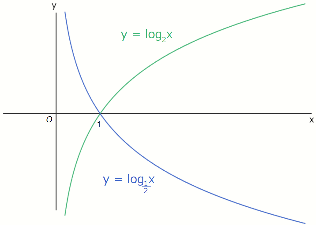
In general, the graphs of \( y = \log _a x \) and \( y = \log _{\frac{1}{a}} x \) are symmetric with
respect to the \( x \)-axis.
Kaya
Well then, let's wrap it up for today.
Nayumi
Good job!
References:
[1] James R. Newman, THE UNIVERSAL ENCYCLOPEDIA OF MATHEMATICS, George Allen & Unwin Ltd, 1964
[2] 石村園子, やさしく学べる微分積分, 共立出版, December 25, 1999
Previous
Ep. 4
Trigonometric function
Trigonometric function
Next

Ep. 6
Derivative of a function of one variable
Derivative of a function of one variable