TABLE OF CONTENTS
・Definite integral
・Calculating area using definite integrals
・Separation of Variables and Definite Integrals
Mathematics articles that help in reading this article
・Numerical Computation:Ep. 1, Ep. 2, Ep. 6, Ep. 8
・Numerical Computation:Ep. 1, Ep. 2, Ep. 6, Ep. 8
Kaya
This time, let’s explain definite integrals.
Definite integral
Nayumi
Definite integrals? How are they different from indefinite integrals?
Kaya
An indefinite integral is an operation that finds a general expression for an antiderivative. In
contrast, a definite integral is obtained by substituting two specific values into an antiderivative and
taking the difference.
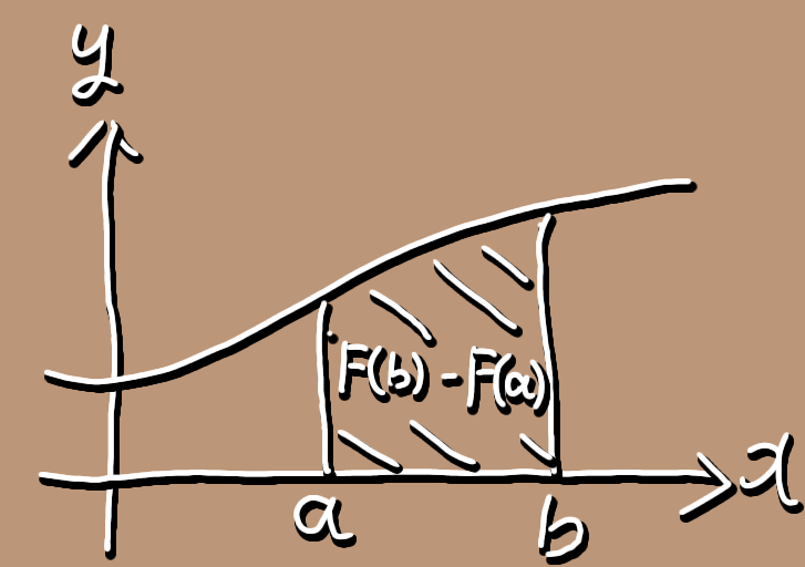
\[ \text{Definite integral}\]
Let \( F(x) \) be one of the antiderivative of the function \( f(x) \).
In this case, \( F(b) - F(a) \) is called the definite integral from \( a \) to \( b \) of \(
f(x) \), and is denoted by
\[ \int ^b _a f(x) dx ,\]
where \( a \) is called the lower limit (or lower bound) of integration, and \( b \) is
called the upper limit (or upper bound) of integration.
In addition, \( F(b) - F(a) \) is denoted as \( \left[ F(x) \right] ^b _a \).
Formulas that hold for indefinite integrals also hold for definite integrals.
For definite integrals, the following formula holds:
\[ \frac{d}{dx} \int ^x _a f(t)dt = f(x) \ \ \left( a \ \text{is constant} \right) \]
\[ \int ^b _a c f(x)dx = c \int ^b _a f(x)dx \ \ \left( c \ \text{is constant} \right) \]
\[ \int ^b _a \left\{ f(x) \pm g(x) \right\} dx = \int ^b _a f(x)dx \pm \int ^b _a g(x)dx \]
Nayumi
It feels like we’ve seen similar formulas before.
Kaya
Yeah. Let’s take this as practice with definite integrals and prove them one by one, starting from the
top.
\[ \begin{align}
\frac{d}{dx} \int ^x _a f(t)dt &= \frac{d}{dx} \left[ F(t) \right] ^x _a \\\\
&= \frac{d}{dx} \left( F(x) - F(a) \right) \\\\
&= f(x)
\end{align}\]
Kaya
Next is the second formula, the constant multiple rule.
\[ \begin{align}
\int ^b _a c f(x)dx &= \left[ cF(x) \right] ^b _a \\\\
&= \left( cF(b) - cF(a) \right) \\\\
&= c \left( F(b) - F(a) \right) \\\\
&= c \int ^b _a f(x)dx
\end{align}\]
Nayumi
And finally, the sum and difference formulas.
\[ \begin{align}
\int ^b _a \left\{ f(x) \pm g(x) \right\} dx &= \left[ F(x) \pm G(x) \right] ^b _a \\\\
&= \left( F(b) \pm G(b) \right) - \left( F(a) \pm G(a) \right) \\\\
&= \left( F(b) - F(a) \right) \pm \left( G(b) - G(a) \right) \\\\
&= \int ^b _a f(x)dx \pm \int ^b _a g(x)dx
\end{align}\]
Kaya
So far, these three formulas also held for indefinite integrals, but there are three more that are
characteristic of definite integrals.
For definite integrals, the following formula holds:
\[ \int ^a _a f(x)dx = 0\]
\[ \int ^b _a f(x)dx = - \int ^a _b f(x)dx\]
\[ \int ^b _a f(x)dx = \int ^c _a f(x)dx + \int ^b _c f(x)dx\]
Nayumi
Hmm, these look like they should be easy to prove too.
Kaya
Right. Let’s start with the first one, the formula for when the lower and upper limits are equal.
\[ \int ^a _a f(x)dx = F(a) - F(a) = 0 \]
Nayumi
Next is the formula where the lower and upper limits are reversed.
\[ \begin{align}
\int ^b _a f(x)dx &= F(b) - F(a) \\\\
&= - \left( F(a) - F(b) \right) \\\\
&= - \int ^a _b f(x)dx
\end{align}\]
Kaya
And finally, the formula for splitting the interval of integration.
\[ \begin{align}
\int ^b _a f(x)dx &= F(b) - F(a) \\\\
&= \left( F(c) - F(a) \right) + \left( F(b) - F(c) \right) \\\\
&= \int ^c _a f(x)dx + \int ^b _c f(x)dx
\end{align}\]
Kaya
Also, substitution works for definite integrals as well.
\[ \text{Integration by substitution}\]
If \( x = g(u) \) is differentiable on the real interval \( \left[ \alpha , \beta \right] \), and \( a
= g \left( \alpha \right) \) and \( b = g \left( \beta \right) \) then the following equation holds:
\[ \begin{align}
\int _a ^b f(x) dx = \int _{\alpha} ^{\beta} f \left( g \left( u \right) \right) g'(u) du.
\end{align}\]
The proof is as follows.
Let \( x = g(u) \).
\[ \begin{align}
\int _{\alpha} ^{\beta} f \left( g \left( u \right) \right) g'(u) du &= \left[ F \left( g \left( u
\right) \right) \right] _{\alpha} ^{\beta} \\\\
&= F \left( g \left( \beta \right) \right) - F \left( g \left( \alpha \right) \right) \\\\
&= F \left( b \right) - F \left( a \right) \\\\
&= \int _a ^b f(x)dx
\end{align}\]
Nayumi
Integration by parts too, right?
\[ \text{Integration by parts}\]
If both \( f(x) \) and \( g(x) \) is differentiable on the real interval \( \left[ a,b \right] \), then
the following equation holds:
\[ \begin{align}
\int _a ^b f(x) g'(x) dx = \left[f(x)g(x) \right] ^b _a - \int _a ^b f'(x) g(x) dx.
\end{align}\]
The proof is as follows.
\[ \begin{align}
\int _a ^b f(x) g'(x) dx + \int _a ^b f'(x) g(x) dx &= \int _a ^b \left\{ f(x) g'(x) + f'(x) g(x)
\right\} dx \\\\
&= \int _a ^b \left\{ f(x) g(x) \right\}' dx \\\\
&= \left[f(x)g(x) \right] ^b _a
\end{align}\]
Therefore,
\[ \begin{align}
\int _a ^b f(x) g'(x) dx = \left[f(x)g(x) \right] ^b _a - \int _a ^b f'(x) g(x) dx
\end{align}\]
Kaya
Okay then, next let’s use definite integrals to find areas.
Calculating area using definite integrals
Nayumi
By area, you mean area like the area of a square, right?
Kaya
Yes, that kind of area. Using definite integrals, we can find the area of a region on the \( xy
\)-coordinate plane enclosed by two functions and two lines parallel to the \( y \)-axis.
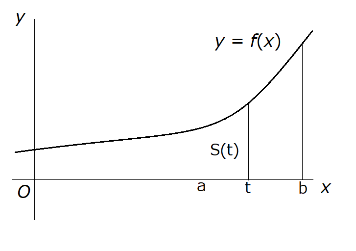
First, on the real interval \( \left[ a,b \right] \), assuming \( f(x) \geq 0 \), let us find the area \(
S(t) \) of the region enclosed by the graph of \( y = f(x) \), the \( x \)-axis, and the two lines \( x = a
\) and \( x = t \ \left( a \leq t \leq b \right) \).
Consider the change in area when \( x \) moves from \( t \) to \( t+h \),
\[ S(t+h) - S(t). \]
This represents the area of the region enclosed by the graph of \( y = f(x) \), the \( x \)-axis, and the
two lines \( x = t \) and \( x = t+h \).
Over the real interval \( \left[ t,t+h \right] \), we can construct a rectangle that has the same area as
this region.
As shown in the figure below, this rectangle can be constructed by choosing the top side so that the two
light-blue shaded regions have equal area.
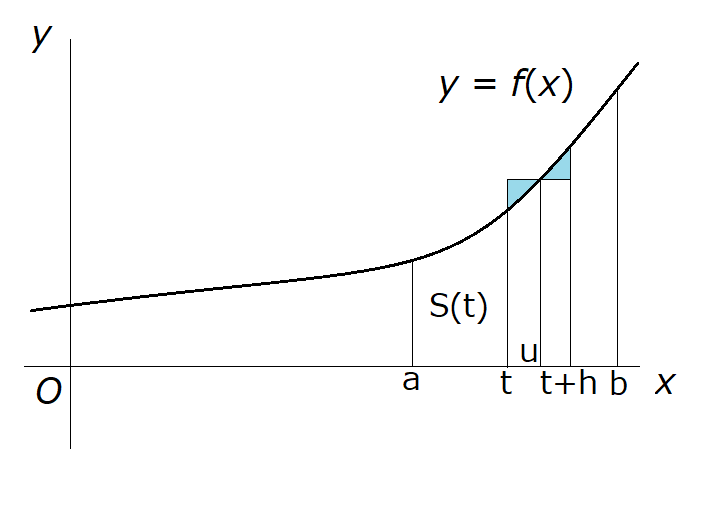
Since the top side of the rectangle must intersect the curve \( y = f(x) \), let \( u \) be the \( x
\)-coordinate of that intersection point. Then the height of the rectangle is given by \( f(u) \).
Therefore, because the change in area is equal to the area of the rectangle, the following equation holds.
\[ \begin{align}
S(t+h) - S(t) &= f(u)h \\\\
\frac{S(t+h) - S(t)}{h} &= f(u)
\end{align}\]
Nayumi
It’s starting to look a bit like a derivative, isn’t it?
Kaya
Good intuition. Here, if we take the limit as \( h \to 0 \), then \( u \to t \) , so the following
holds.
\[ \begin{align}
\lim _{h \to 0} \frac{S(t+h) - S(t)}{h} &= \lim _{h \to 0} f(u) \\\\
S'(t) &= f(t)
\end{align}\]
We have found that \( S(t) \) is an antiderivative of \( f(t) \).
After rewriting the variable on both sides as \( x \ \left( a \leq x \leq b \right) \), and then taking the
definite integral with respect to \( x \) from the lower limit \( a \) to the upper limit \( t \), we obtain
the following expression, since \( S(a)=0 \).
\[ \begin{align}
S'(x) &= f(x) \\\\
\int _a ^t S'(x) dx &= \int _a ^t f(x) dx \\\\
S(t) - S(a) &= \int _a ^t f(x) dx \\\\
S(t) &= \int _a ^t f(x) dx
\end{align}\]
Nayumi
Okay, so now we’ve expressed the area enclosed by the graph of \( y = f(x) \), the \( x \)-axis, and the
two lines \( x = a \) and \( x = t \) using a definite integral.
Kaya
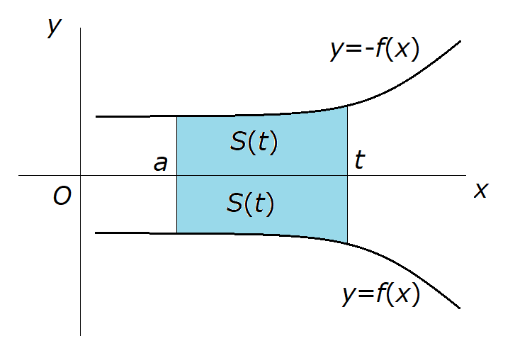
Exactly. Next, let’s find the area in the same way for the case where \( f(x) \leq 0 \) on the real
interval \( \left[ a,b \right] \).
In the case where \( f(x) \leq 0 \), we can carry out the same argument by applying the previous formula to
the function \( y = -f(x) \), which is the reflection of \( y = f(x) \) across the \( x \)-axis.
\[ \begin{align}
S(t) &= \int _a ^t \left\{ -f(x) \right\} dx = - \int _a ^t f(x) dx
\end{align}\]
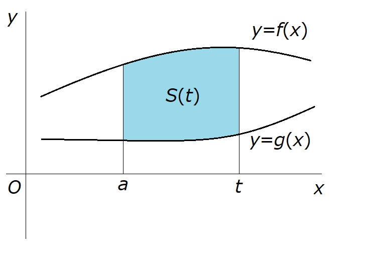
Finally, in the general case, suppose that two functions \( y = f(x) \) and \( y = g(x) \) satisfy \( f(x)
\geq g(x) \) on the real interval \( \left[ a,b \right] \).
We seek the area \( S(t) \) of the region enclosed by \( y = f(x) \), \( y = g(x) \), and the lines \( x=a
\) and \( x = t \ \left( a \leq t \leq b \right)\).
First, let us consider the case where \( g(x) \geq 0 \) on the real interval \( \left[ a,b \right] \).
First, let us consider the case where \( g(x) \geq 0 \) on the real interval \( \left[ a,b \right] \).
Nayumi
Wouldn’t it work to cut out the lower part from the whole?
Kaya
Nice idea. Using that approach, \( S(t) \) can be expressed by the following formula.
\[ \begin{align}
S(t) &= \int _a ^t f(x) dx - \int _a ^t g(x) dx \\\\
&= \int _a ^t \left\{ f(x) - g(x) \right\} dx
\end{align}\]
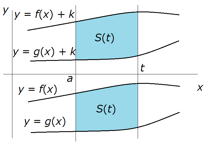
Next, consider the case where \( g(x) \lt 0 \) on the real interval \( \left[ a,b \right] \).
In this case, we can choose a constant \( k \) such that \( g(x) + k \geq 0 \), and then consider the two
functions shifted upward in the \( y \)--direction by \( +k \), namely \( y = f(x) + k \) and \( y = g(x) +
k \).
Since this does not change the area, the following formula holds.
\[ \begin{align}
S(t) &= \int _a ^t \left\{ f(x) + k \right\} dx - \int _a ^t \left\{ g(x) + k \right\} dx \\\\
&= \int _a ^t \left\{ f(x) - g(x) \right\} dx
\end{align}\]
Nayumi
In the end, it turns out to be the same formula as before.
Kaya
Exactly. That wraps up our discussion of definite integrals and area. Finally, let’s take a look at one
point regarding the method of separation of variables.
Separation of Variables and Definite Integrals
Nayumi
We’ve always used indefinite integrals in the method of separation of variables, haven’t we?
Kaya
That’s right. But about that usual solution method—you can actually do the same thing using definite
integrals.
When we use indefinite integrals to apply the method of separation of variables, we determine the specific
value of the constant of integration afterward by using the initial condition.
On the other hand, when we use definite integrals, we can solve the problem in one step by incorporating the
initial condition as the lower limit of the integral.
Comparing the two approaches, it looks like this.
Consider an ordinary differential equation involving the functions \( p(x) \) and \( q(y) \),
\[ q(y) dy = p(x) dx. \]
We solve it in two different ways. Let \( P(x) \) and \( Q(y) \) be antiderivatives of \( p(x) \) and \(
q(y) \), respectively, and let the initial condition be \( \left( x_0, y_0 \right) \).
(1) Method using indefinite integrals \[ \begin{align} q(y) dy &= p(x) dx \\\\ \int q(y) dy &= \int p(x) dx \\\\ Q(y) &= P(x) + C \\\\ \end{align}\] From the initial condition, \[ C = Q(y_0) - P(x_0) \] Therefore, \[ \begin{align} Q(y) &= P(x) + Q(y_0) - P(x_0) \\\\ Q(y) - Q(y_0) &= P(x) - P(x_0) \end{align}\]
(2) Method using definite integrals \[ \begin{align} q(y) dy &= p(x) dx \\\\ \int ^y _{y_0} q(y) dy &= \int ^x _{x_0} p(x) dx \\\\ Q(y) - Q(y_0) &= P(x) - P(x_0) \\\\ \end{align}\]
Nayumi
It really does give the same result either way. The method using definite integrals takes fewer lines,
doesn’t it?
Kaya
What we’re doing is the same, though. From now on, we’ll probably also use descriptions based on
definite integrals in numerical experiments.
Nayumi
Got it.
Kaya
Alright then, let’s stop here for today.
References:
[1] 宮西正宜 23 others, 高等学校 数学Ⅱ 改訂版, 新興出版社啓林館, December 10, 2009
Previous
Ep. 12
Bisection method and Newton's method
Bisection method and Newton's method
Next
Ep. 14
Set
Set